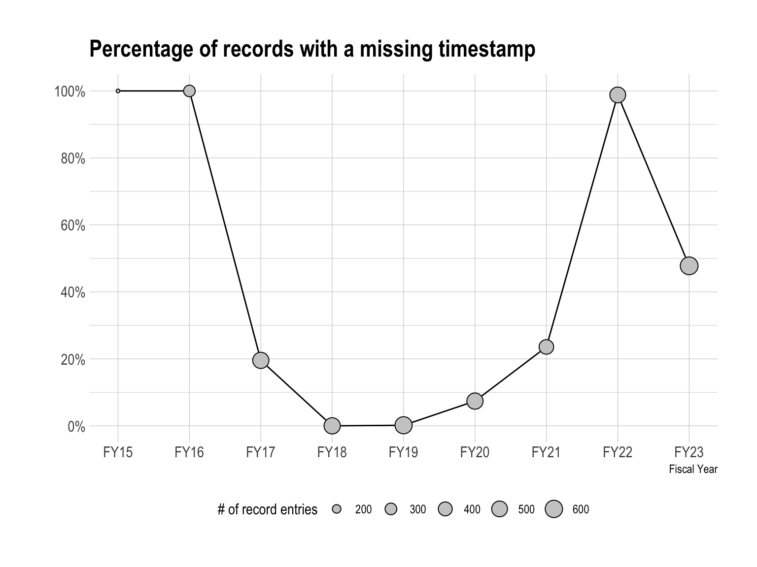
The first theme to emerge from data exploration was data completeness. Missing values were most prominent for timestamp variables such as
the datetime the Office of Sponsored Projects was notified of about the status of the award and
the datetime the award was actionedon by the Office of Sponsored Projects.
Timestamps are an integral data point because they allows us to track the lifecycle of an award as well as compute the duration of time an award spends in any given phase of the lifecycle. Without timestamp data, it is increasingly difficult to gain a comprehensive understanding of processes and improve them from a data-informed approach.
Researchers have stated that bias is likely in analyses with more than 10% missingness and that more than 40% missing data means we can only postulate but draw no firm conclusions. (Dowd et. al, 2019). The visualization below shows that timestamp variables were missing at critical levels prior to and after the Covid-19 pandemic.
The significant missingness of timestamp data meant my analysis would stop short of making conclusion with statistical significance as well as limit the possibility of finding definitive trends. Despite this, the subsequent analysis still sheds some light into our workflows and provides a starting framework for how this research might continue going forward.
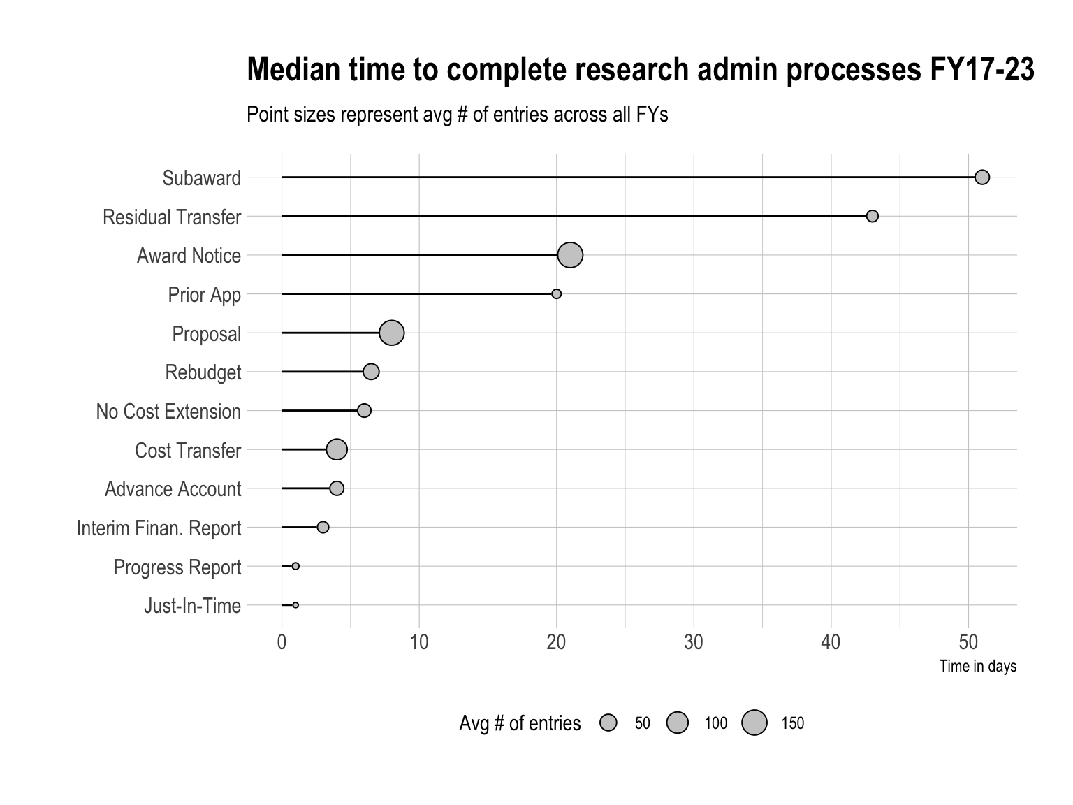
Process efficiency
The figure below visualizes the typical time to complete each task from FY17-23. Across all fiscal years, subawards have shown to take the longest to complete with an expected completion of around 50 days. It’s worth noting that across all fiscal years, CEHD also processes about 50 subawards each year.
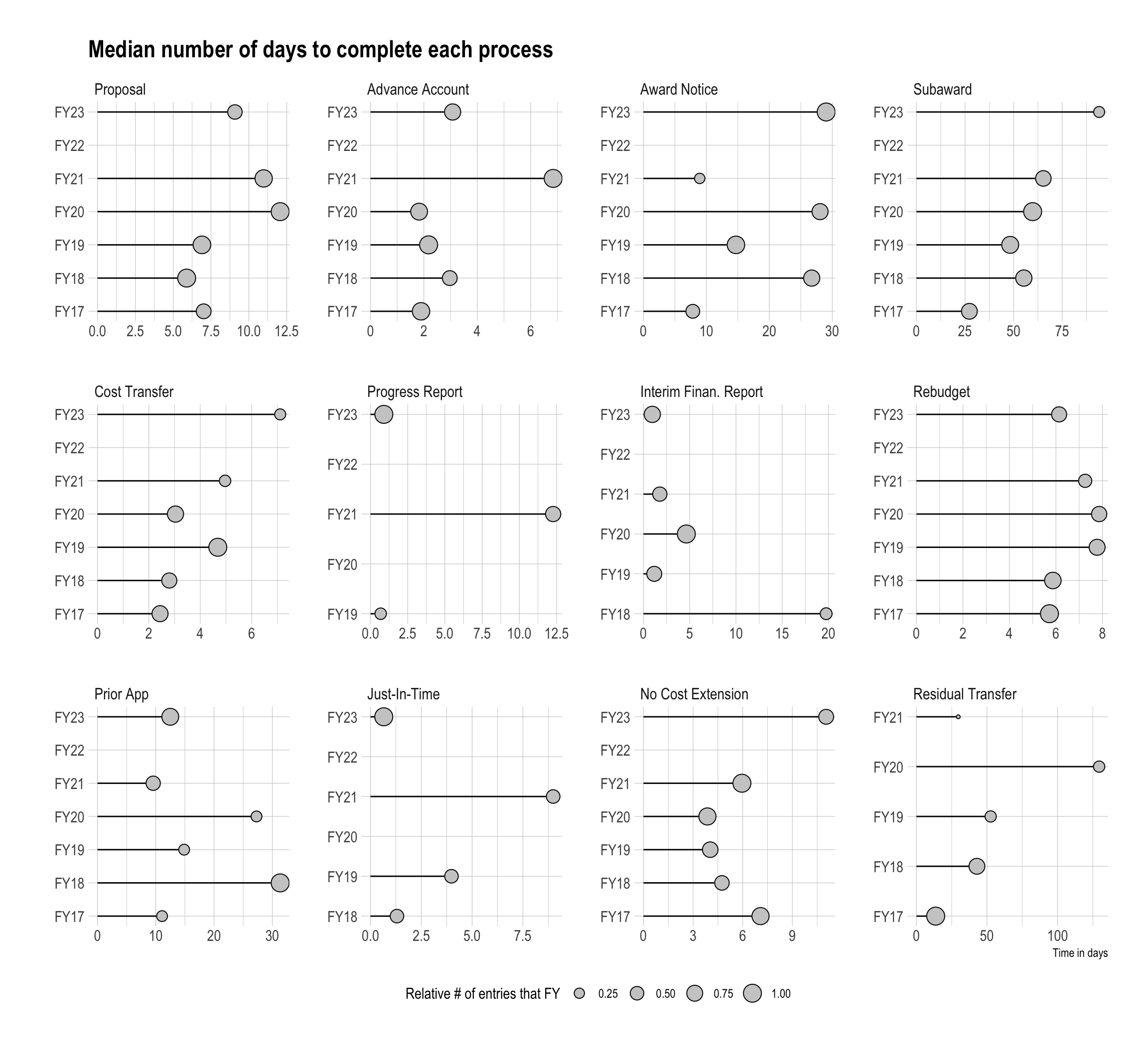
The figure below shows us a breakdown of process times for each workflow across all fiscal years.
Proposals
In order to reach GSU’s goal of doubling it’s research expenditures by the next decade, one of the first milestones we must inevitably reach is increasing our number of proposals. The logic here being that as the numbers of proposals increase, then the number of awards will (hopefully) also tend to increase. However, the path to a proposal’s acceptance begins long before it reaches the sponsor. Proposals must first be reviewed, approved, and submitted to the sponsor by the Office of Sponsored Projects and Awards (OSPA), ideally days before the deadline so that OSPA can conduct a diligent review.
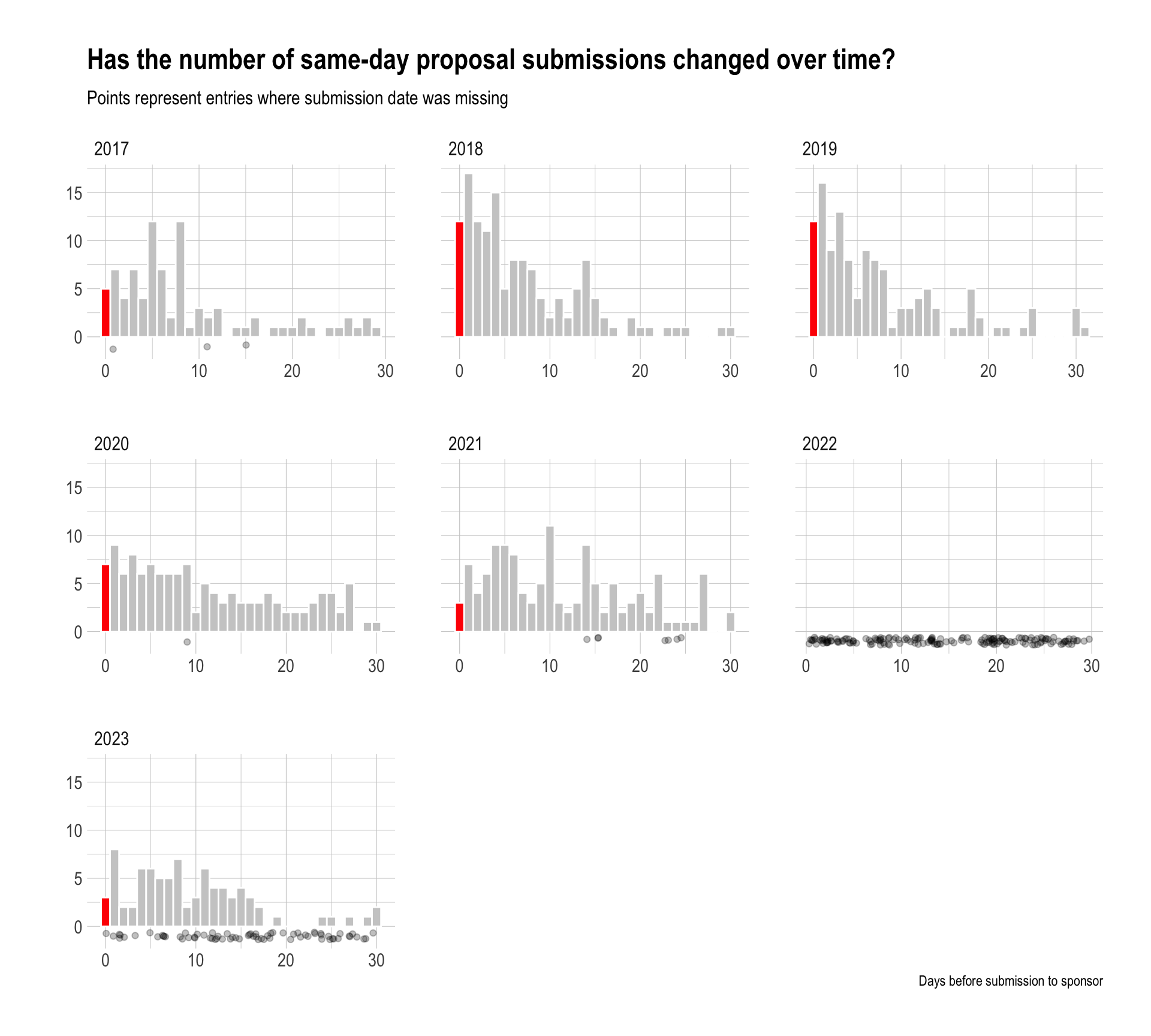
The number of same-day submissions in CEHD peaked in FY19 with approximately 9.68% of proposal being submitted to the sponsor the same day they were received by OSPA. Soon thereafter, OSPA implemented a policy that said proposals should be submitted five days in advance of the proposal due date to allow sufficient time for review. But did that policy have an effect?
At first glance, it appears that the policy did have a positive effect on decreasing same-day submissions as evidenced by the decreasing red lines in the figure below. In FY23, the percentage drops to as low as 3.66%. However, recall that nearly 100% of timestamp data were missing in FY22 and approximately 50% of the timestamp data were missing in FY23. Therefore, these values are removed from our sample (as evidenced by the dots in the visualization below which have no value). Given that those durations could be anything (including same-day submissions), it is impossible to draw any conclusions on whether we have made progress on this front.
The fact remains, submitting proposals to OSPA is a requirement and them being submitted early is also necessary. If we are to meet our 10-year strategic goals, I believe we must first invest in an infrastructure that empowers PIs to submit proposals both early and often.
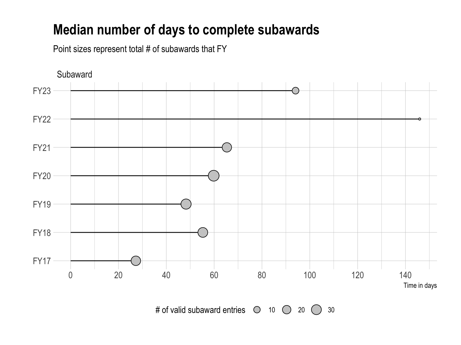
Subawards
Subawards is yet another contentious area of research administration. Best practice says that subawards should be set up within ~30 days. However, in FY23 we see that process took as long as 90 days in some instances.
Completing a subaward 90 days after the initial award set up is well beyond the 30-day best practice. When you couple in the fact that subawardees often begin their research well before the award set up but can’t be reimbursed, we get a greater sense of the compounding effects that this bottleneck has on the system. Additionally, it’s reasonable to assume that a process this insufficient can have a negative impact on recruiting and retaining both faculty and research administrators from considering GSU as their home.
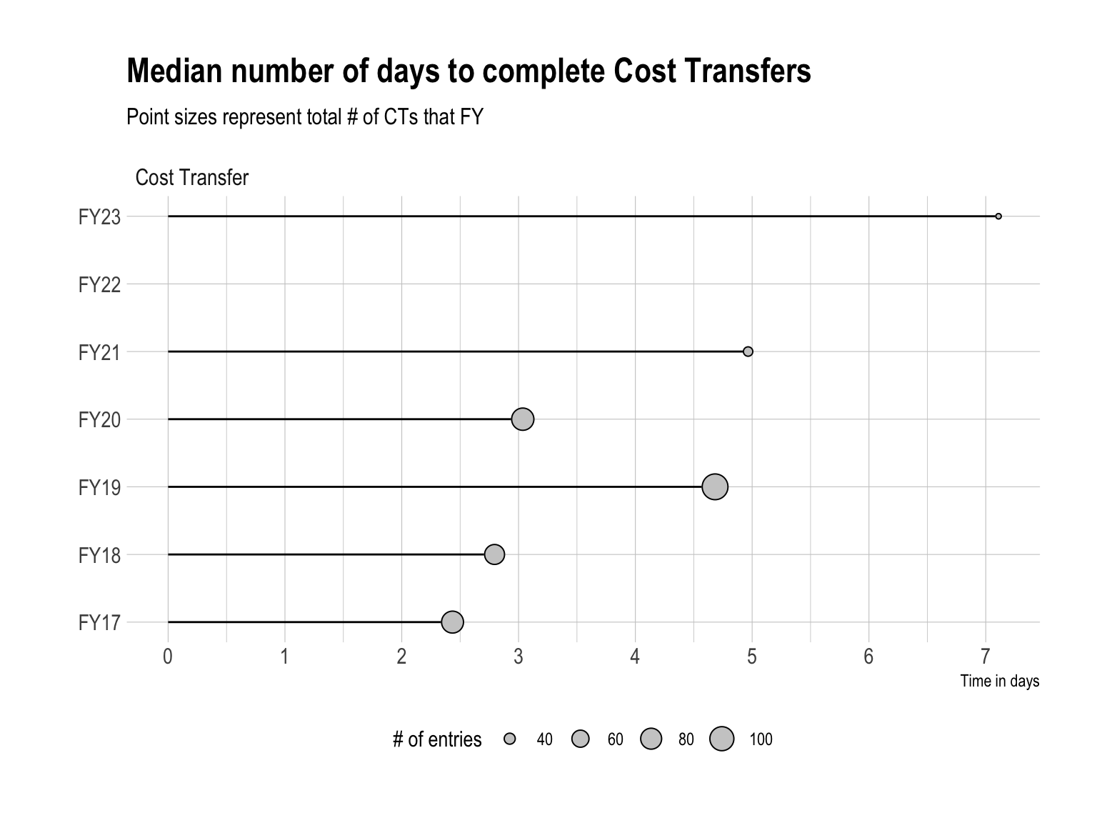
Cost Transfers
This analysis of GSU’s research administration processes ends with cost transfers. One highlight within the data is that in FY23, CEHD recorded its lowest number of cost transfers for a total of 34. However, despite this decrease, interestingly we also see that cost transfers are tending to take longer to complete, M = 7 days in FY23. This might suggest that our research administrators are getting better at catching budget discrepancies before its too late.
Despite this fewer numbers of cost transfers, we also see that cost transfers may be tending to take longer to process over time. (Recall, given the significant missingness of the data, we must be careful not to make definitive conclusions). If this is in fact true, this may be due to the fact that some PIs are doing a worse job of reviewing their expenses and these may be the most complex cost transfers to process.
Source Code
---title: ""execute: echo: false warning: falseformat: html: code-tools: source: true toggle: false caption: noneeditor_options: chunk_output_type: console---```{r global options, include = FALSE}knitr::opts_chunk$set(message=FALSE)``````{r load-libraries-data}library(tidyverse)library(scales)library(janitor)library(readxl)library(lubridate)library(tidytext)library(gridExtra)library(knitr)library(hrbrthemes)library(qrcode)library(naniar)library(bookdown)theme_set(theme_ipsum())research_portal <-read_csv("data/clean/research_portal_clean.csv") %>%mutate(con_number =as.factor(con_number))missing <-read_csv("data/clean/missing.csv")research_portal_summary <-read_csv("data/clean/research_portal_summary.csv") %>%mutate(submission_type =as.factor(submission_type))```# Data Integrity## CompletenessThe first theme to emerge from data exploration was **data completeness**. Missing values were most prominent for timestamp variables such as1. the datetime the **Office of Sponsored Projects was [notified]{.underline}** of about the status of the award and2. the datetime the award was [**actioned**]{.underline} **on by the Office of Sponsored Projects**.Timestamps are an integral data point because they allows us to track the lifecycle of an award as well as compute the duration of time an award spends in any given phase of the lifecycle. Without timestamp data, it is increasingly difficult to gain a comprehensive understanding of processes and improve them from a data-informed approach.Researchers have stated that bias is likely in analyses with more than 10% missingness and that more than 40% missing data means we can only postulate but draw no firm conclusions. ([Dowd et. al, 2019](https://www.sciencedirect.com/science/article/pii/S0895435618308710#:~:text=Statistical%20guidance%20articles%20have%20stated,18%5D%2C%20%5B19%5D. "Dowd et. al, 2019")). The visualization below shows that timestamp variables were missing at critical levels prior to and after the Covid-19 pandemic.```{r missing-data-vis}#| fig-width: 8#| fig-height: 6research_portal %>%filter(!is.na(fiscal_year)) %>%group_by(fiscal_year, fy_labels) %>%summarise(n_entries =n(),n_dates_missing =sum(is.na(osp_received) |is.na(last_modified)),pct_dates_missing = n_dates_missing/n_entries ) %>%ggplot(aes(x = fiscal_year, y = pct_dates_missing)) +geom_line() +geom_point(aes(size = n_entries), color ="grey80") +geom_point(aes(size = n_entries), pch =21) +scale_x_continuous(breaks =seq(2015, 2023, 1),labels =c("FY15", "FY16", "FY17", "FY18", "FY19", "FY20", "FY21", "FY22", "FY23"),minor_breaks =NULL) +scale_y_continuous(labels = scales::percent_format(),breaks =seq(0, 1, .2)) +labs(x ="Fiscal Year",y ="",title ="Percentage of records with a missing timestamp", size ="# of record entries") +theme(legend.position ="bottom")```The significant missingness of timestamp data meant my analysis would stop short of making conclusion with statistical significance as well as limit the possibility of finding definitive trends. Despite this, the subsequent analysis still sheds some light into our workflows and provides a starting framework for how this research might continue going forward.# Process efficiencyThe figure below visualizes the typical time to complete each task from FY17-23. Across all fiscal years, subawards have shown to take the longest to complete with an expected completion of around 50 days. It's worth noting that across all fiscal years, CEHD also processes about 50 subawards each year.```{r}#| fig-width: 8#| fig-height: 6research_portal %>%filter(!is.na(duration_days)) %>%group_by(submission_type) %>%summarise(avg_entries_fy =mean(n_entries_fy, na.rm = T),median_duration_days =median(duration_days, na.rm = T)) %>%mutate(submission_type =fct_reorder(submission_type, median_duration_days, "sum")) %>%ggplot(aes(x = submission_type, y = median_duration_days)) +geom_segment(aes(x=submission_type, xend=submission_type, y=0, yend=median_duration_days)) +geom_point(aes(size = avg_entries_fy), color ="grey80", fill ="grey20") +geom_point(aes(size = avg_entries_fy), pch =21) +coord_flip() +labs(x ="",y ="Time in days",title ="Median time to complete research admin processes FY17-23",subtitle ="Point sizes represent avg # of entries across all FYs",size ="Avg # of entries") +theme(legend.position ="bottom")```The figure below shows us a breakdown of process times for each workflow across all fiscal years. ```{r}#| fig-width: 12#| fig-height: 11research_portal_summary <- research_portal %>%group_by(submission_type, submission_type_numeric, fiscal_year, fy_labels) %>%summarise(n_entries =sum(!is.na(duration_days)),median_duration_sec =median(duration, na.rm = T),median_duration_days =as.numeric(median_duration_sec)/86400,.groups ="drop") %>%group_by(submission_type) %>%mutate(point_size =rescale(n_entries, to =c(0,1))) %>%arrange(submission_type, n_entries)research_portal_summary %>%filter(!is.na(median_duration_days), fiscal_year !=2022) %>%mutate(submission_type =fct_reorder(submission_type, submission_type_numeric)) %>%ggplot(aes(x = fiscal_year, y = median_duration_days)) +geom_segment(aes(x=fiscal_year, xend=fiscal_year, y=0, yend=median_duration_days)) +geom_point(aes(size = point_size), color ="grey80", fill ="grey20") +geom_point(aes(size = point_size), pch =21) +scale_x_continuous(breaks =seq(2015, 2023, 1), minor_breaks =NULL,labels =c("FY15", "FY16", "FY17", "FY18", "FY19", "FY20", "FY21", "FY22", "FY23")) +facet_wrap(~ submission_type %>%fct_reorder(submission_type_numeric), scales ="free") +coord_flip() +expand_limits() +labs(x ="",y ="Time in days",title =str_wrap("Median number of days to complete each process",width =50),# subtitle = "Point sizes represent relative # of entries that FY",size ="Relative # of entries that FY") +theme(legend.position ="bottom")``````{r}same_day_submissions_2019 <- research_portal %>%filter(submission_type =="Proposal", fiscal_year ==2019, duration_days ==0) %>%nrow() all_submissions_2019 <- research_portal %>%filter( submission_type =="Proposal", fiscal_year ==2019, duration_days <=31) %>%nrow() %>%round(2) pct_same_day_submissions_2019 <- ((same_day_submissions_2019 / all_submissions_2019) *100) %>%round(2)same_day_submissions_2023 <- research_portal %>%filter(submission_type =="Proposal", fiscal_year ==2023, duration_days ==0) %>%nrow()all_submissions_2023 <- research_portal %>%filter(submission_type =="Proposal", fiscal_year ==2023, duration_days <=31) %>%nrow()pct_same_day_submissions_2023 <- ((same_day_submissions_2023/ all_submissions_2023) *100) %>%round(2)```## ProposalsIn order to reach GSU's goal of doubling it's research expenditures by the next decade, one of the first milestones we must inevitably reach is increasing our number of proposals. The logic here being that as the numbers of proposals increase, then the number of awards will (*hopefully*) also tend to increase. However, the path to a proposal's acceptance begins long before it reaches the sponsor. Proposals must first be reviewed, approved, and submitted to the sponsor by the Office of Sponsored Projects and Awards (OSPA), ideally days before the deadline so that OSPA can conduct a diligent review.The number of same-day submissions in CEHD peaked in FY19 with approximately `r pct_same_day_submissions_2019`% of proposal being submitted to the sponsor the same day they were received by OSPA. Soon thereafter, OSPA implemented a policy that said proposals should be submitted five days in advance of the proposal due date to allow sufficient time for review. But did that policy have an effect?```{r proposal-histogram, fig.width = 10, fig.height=9}colors <-c(rep("red", 1), rep("grey80", 29), rep("red", 1), rep("grey80", 30), rep("red", 1), rep("grey80", 31),rep("red", 1), rep("grey80", 30), rep("red", 1), rep("grey80", 30), rep("red", 1), rep("grey80", 30))research_portal_histogram <- research_portal %>%filter(fiscal_year >2016)ggplot() +geom_histogram(data = research_portal_histogram %>%filter(submission_type =="Proposal", duration_days <=31), mapping =aes(x = duration_days), binwidth =1, color ="white",fill = colors) +geom_jitter(data = research_portal_histogram %>%filter(submission_type =="Proposal") %>%mutate(osp_received =if_else(is.na(osp_received), 15, NA)) %>%group_by(submission_type), aes(x = osp_received, y =-1), alpha = .25, width =15) +facet_wrap(~ fiscal_year, "free_x",nrow =NULL, ncol =NULL) +#scale_x_continuous() +labs(x ="Days before submission to sponsor",y ="",title ="Has the number of same-day proposal submissions changed over time?",subtitle ="Points represent entries where submission date was missing")```At first glance, it appears that the policy did have a positive effect on decreasing same-day submissions as evidenced by the decreasing red lines in the figure below. In FY23, the percentage drops to as low as `r pct_same_day_submissions_2023`%. However, recall that nearly 100% of timestamp data were missing in FY22 and approximately 50% of the timestamp data were missing in FY23. Therefore, these values are removed from our sample (as evidenced by the dots in the visualization below which have no value). Given that those durations could be anything (including same-day submissions), it is impossible to draw any conclusions on whether we have made progress on this front. The fact remains, submitting proposals to OSPA is a requirement and them being submitted early is also necessary. If we are to meet our 10-year strategic goals, I believe we must first invest in an infrastructure that empowers PIs to submit proposals both early and often.## SubawardsSubawards is yet another contentious area of research administration. Best practice says that subawards should be set up within ~30 days. However, in FY23 we see that process took as long as 90 days in some instances.```{r fig.width = 8, fig.height=6}research_portal_summary %>%filter(!is.na(median_duration_days), submission_type =="Subaward") %>%mutate(submission_type =fct_reorder(submission_type, median_duration_sec)) %>%ggplot(aes(x = fiscal_year, y = median_duration_days)) +geom_segment(aes(x=fiscal_year, xend=fiscal_year, y=0, yend=median_duration_days)) +geom_point(aes(size = n_entries), color ="grey80", fill ="grey20") +geom_point(aes(size = n_entries), pch =21) +scale_x_continuous(breaks =seq(2017, 2023, 1),labels =c("FY17", "FY18", "FY19", "FY20", "FY21", "FY22", "FY23"),minor_breaks =NULL) +scale_y_continuous(breaks =seq(0, 140, 20)) +facet_wrap(~ submission_type, scales ="free") +coord_flip() +labs(x ="",y ="Time in days",title ="Median number of days to complete subawards",subtitle ="Point sizes represent total # of subawards that FY",size ="# of valid subaward entries") +theme(legend.position ="bottom")```Completing a subaward 90 days after the initial award set up is well beyond the 30-day best practice. When you couple in the fact that subawardees often begin their research well before the award set up but can't be reimbursed, we get a greater sense of the compounding effects that this bottleneck has on the system. Additionally, it's reasonable to assume that a process this insufficient can have a negative impact on recruiting and retaining both faculty and research administrators from considering GSU as their home.## Cost Transfers```{r}ct_entries_2023 <- research_portal_summary %>%filter(submission_type =="Cost Transfer", fiscal_year ==2023) %>%pull(n_entries)ct_durations_2023 <- research_portal_summary %>%filter(submission_type =="Cost Transfer", fiscal_year ==2023) %>%pull(median_duration_days) %>%round(0)```This analysis of GSU's research administration processes ends with cost transfers. One highlight within the data is that in FY23, CEHD recorded its lowest number of cost transfers for a total of `r ct_entries_2023`. However, despite this decrease, interestingly we also see that cost transfers are tending to take longer to complete, M = `r ct_durations_2023` days in FY23. This might suggest that our research administrators are getting better at catching budget discrepancies before its too late. Despite this fewer numbers of cost transfers, we also see that cost transfers *may* be tending to take longer to process over time. (Recall, given the significant missingness of the data, we must be careful not to make definitive conclusions). If this is in fact true, this may be due to the fact that some PIs are doing a worse job of reviewing their expenses and these may be the most complex cost transfers to process. ```{r}#| fig-width: 8#| fig-height: 6research_portal_summary %>%#mutate(duration_days = if_else(is.na(duration_days), 0, duration_days)) %>% filter(!is.na(median_duration_days), submission_type =="Cost Transfer") %>%mutate(submission_type =fct_reorder(submission_type, median_duration_sec)) %>%ggplot(aes(x = fiscal_year, y = median_duration_days)) +geom_segment(aes(x=fiscal_year, xend=fiscal_year, y=0, yend=median_duration_days)) +geom_point(aes(size = n_entries), color ="grey80", fill ="grey20") +geom_point(aes(size = n_entries), pch =21) +scale_x_continuous(breaks =seq(2017, 2023, 1),labels =c("FY17", "FY18", "FY19", "FY20","FY21", "FY22", "FY23"),minor_breaks =NULL) +scale_y_continuous(breaks =seq(0,8,1),) +facet_wrap(~ submission_type, scales ="free") +coord_flip() +labs(x ="",y ="Time in days",title ="Median number of days to complete Cost Transfers",subtitle ="Point sizes represent total # of CTs that FY",size ="# of entries") +theme(legend.position ="bottom")``````{r}#| fig-width: 8#| fig-height: 40primary_dept_contacts <-c("Mi'Yata Johnson-Foreman", "Stacy Ringo", "Letitia Williams", "Shaila Philpot")shailas_N_awards <-n_distinct(research_portal %>%ungroup() %>%filter(str_detect(dept_contact, "Philpot"), fiscal_year ==2019, end_date <="2020-06-30") %>%pull(con_number))research_portal %>%mutate(con_number =if_else(is.na(con_number), "Missing Con #", con_number),last_modified = end_date %>%as_date(),submission_type_lumped =fct_lump(submission_type, 6)) %>%filter(dept_contact %in% primary_dept_contacts, fiscal_year ==2020, end_date <="2020-06-30", submission_type_lumped !="Other") %>%group_by(dept_contact) %>%mutate(dept_contact =str_c(dept_contact, ": (", n_distinct(con_number), " Awards)")) %>%ungroup() %>%ggplot(aes(x =as_date(end_date), y = con_number, shape = submission_type_lumped, color = submission_type_lumped,label = submission_type_lumped)) +geom_point(size =4) +#geom_point(data = research_portal %>% filter(submission_type == "Cost Transfer"), size = 5, alpha = .5) +geom_text(color ="black", size =4, vjust =1, hjust =1, check_overlap = T, show.legend ="none") +facet_wrap(~ dept_contact , scales ="free", ncol =1) +scale_x_date(date_labels ="%m-%d-%y") +scale_y_discrete(expand =expansion(mult =0, add =1)) +labs(x ="Last modified",y ="",title ="Project status by department contact",color ="Submission",shape ="Submission",caption =str_c("Various actions for ", shailas_N_awards," awards managed by research admin"), ) +theme(legend.position ="top") ```